Setup

We now start with the economics motivating the model and then turn to the solution and estimation approach. We conclude with a discussion of a simulated example.

Economics

Keane and Wolpin (1994) develop a model in which an agent decides among \(K\) possible alternatives in each of \(T\) (finite) discrete periods of time. Alternatives are defined to be mutually exclusive and \(d_k(t) = 1\) indicates that alternative \(k\) is chosen at time \(t\) and \(d_k(t) = 0\) indicates otherwise. Associated with each choice is an immediate reward \(R_k(S(t))\) that is known to the agent at time \(t\) but partly unknown from the perspective of periods prior to \(t\). All the information known to the agent at time \(t\) that affects immediate and future rewards is contained in the state space \(S(t)\).

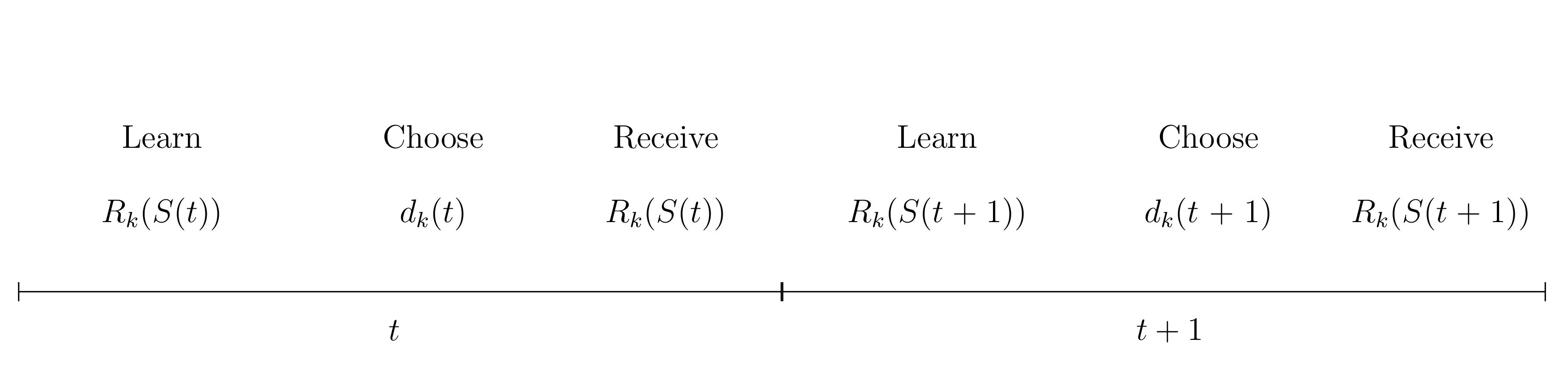
We depict the timing of events below. At the beginning of period \(t\) the agent fully learns about all immediate rewards, chooses one of the alternatives and receives the corresponding benefits. The state space is then updated according to the agent’s state experience and the process is repeated in \(t + 1\).

Agents are forward looking. Thus, they do not simply choose the alternative with the highest immediate rewards each period. Instead, their objective at any time \(\tau\) is to maximize the expected rewards over the remaining time horizon:

\[\max_{\{d_k(t)\}_{k \in K}} E\left[ \sum_{\tau = t}^T \delta^{\tau - t} \sum_{k\in K}R_k(\tau)d_k(\tau)\Bigg| S(t)\right]\]

The discount factor \(0 > \delta > 1\) captures the agent’s preference for immediate over future rewards. Agents maximize the equation above by choosing the optimal sequence of alternatives \(\{d_k(t)\}_{k \in K}\) for \(t = \tau, .., T\).

Within this more general framework, Keane and Wolpin (1994) consider the case where agents are risk neutral and each period choose to work in either of two occupations (\(k = 1,2\)), to attend school (\(k = 3\)), or to remain at home (\(k = 4\)). The immediate reward functions are given by:

\[ \begin{align}\begin{aligned}R_1(t) &= w_{1t} =\exp\{\alpha_{10} + \alpha_{11}s_t + \alpha_{12}x_{1t} - \alpha_{13}x^2_{1t} + \alpha_{14}x_{2t} - \alpha_{15}x^2_{2t} + \epsilon_{1t}\}\\R_2(t) &= w_{2t} =\exp\{\alpha_{20} + \alpha_{21}s_t + \alpha_{22}x_{1t} - \alpha_{23}x^2_{1t} + \alpha_{24}x_{2t} - \alpha_{25}x^2_{2t} + \epsilon_{2t}\}\\R_3(t) &= \beta_0 - \beta_1 I(s_t \geq 12) - \beta_2(1 - d_3(t -1)) + \epsilon_{3t}\\R_4(t) &= \gamma_0 + \epsilon_{4t},\end{aligned}\end{align} \]

where \(s_t\) is the number of periods of schooling obtained by the beginning of period \(t\), \(x_{1t}\) is the number of periods that the agent worked in occupation one by the beginning of period \(t\), \(x_{2t}\) is the analogously defined level of experience in occupation two, \(\alpha_1\) and \(\alpha_2\) are parameter vectors associated with the wage functions, \(\beta_0\) is the consumption value of schooling, \(\beta_1\) is the post-secondary tuition cost of schooling, with \(I\) an indicator function equal to one if the agent has completed high school and zero otherwise, \(\beta_2\) is an adjustment cost associated with returning to school, \(\gamma_0\) is the (mean) value of the non-market alternative. The \(\epsilon_{kt}\)‘s are alternative-specific shocks to occupational productivity, to the consumption value of schooling, and to the value of non-market time. The productivity and taste shocks follow a four-dimensional multivariate normal distribution with mean zero and covariance matrix \(\Sigma = [\sigma_{ij}]\). The realizations are independent across time. We collect the parametrization of the reward functions in \(\theta = \{\alpha_1, \alpha_2, \beta, \gamma, \Sigma\}\).

Given the structure of the reward functions and the agents objective, the state space at time \(t\) is:

\[S(t) = \{s_t,x_{1t},x_{2t}, d_3(t - 1),\epsilon_{1t},\epsilon_{2t},\epsilon_{3t},\epsilon_{4t}\}.\]

It is convenient to denote its observable elements as \(\bar{S}(t)\). The elements of \(S(t)\) evolve according to:

\[ \begin{align}\begin{aligned}x_{1,t+1} &= x_{1t} + d_1(t)\\x_{2,t+1} &= x_{2t} + d_2(t)\\s_{t+1} &= s_{t\phantom{2}} + d_3(t)\\f(\epsilon_{t+1}\mid S(t), d_k(t)) &= f(\epsilon_{t+1}\mid \bar{S}(t), d_k(t)),\end{aligned}\end{align} \]

where the last equation reflects the fact that the \(\epsilon_{kt}\)‘s are serially independent. We set \(x_{1t} = x_{2t} = 0\) as the initial conditions.

Solution

From a mathematical perspective, this type of model boils down to a finite-horizon DP problem under uncertainty that can be solved by backward induction. For the discussion, it is useful to define the value function \(V(S(t),t)\) as a shorthand for the agents objective function. \(V(S(t),t)\) depends on the state space at \(t\) and on \(t\) itself due to the finiteness of the time horizon and can be written as:

\[\begin{align} V(S(t),t) = \max_{k \in K}\{V_k(S(t),t)\}, \end{align}\]

with \(V_k(S(t),t)\) as the alternative-specific value function. \(V_k(S(t),t)\) obeys the Bellman equation (Bellman, 1957) and is thus amenable to a backward recursion.

\[\begin{split}\begin{align} V_k(S(t),t) = \begin{cases} R_k(S(t)) + \delta E\left[V(S(t + 1), t + 1) \mid S(t), d_k(t) = 1\right] &\qquad\mbox{if } t < T \\ R_k(S(t)) &\qquad\mbox{if } t = T. \end{cases} \end{align}\end{split}\]

Assuming continued optimal behavior, the expected future value of state \(S(t + 1)\) for all \(K\) alternatives given today’s state \(S(t)\) and choice \(d_k(t) = 1\), \(E\max(S(t + 1))\) for short, can be calculated:

\[E\max(S(t + 1)) = E\left[V(S(t + 1), t + 1) \mid S(t), d_k(t) = 1\right].\]

This requires the evaluation of a \(K\) - dimensional integral as future rewards are partly uncertain due to the unknown realization of the shocks:

\[ \begin{align}\begin{aligned} E\max(S(t)) =\hspace{11cm}\\\int_{\epsilon_1(t)} ... \int_{\epsilon_K(t)}\max\{R_1(t), ..., R_K(t)\}f_{\epsilon}(\epsilon_1(t), ... ,\epsilon_K(t))d\epsilon_1(t) ... d\epsilon_K(t),\end{aligned}\end{align} \]

where \(f_{\epsilon}\) is the joint density of the uncertain component of the rewards in \(t\) not known at \(t - 1\). With all ingredients at hand, the solution of the model by backward induction is straightforward.

Estimation

We estimate the parameters of the reward functions \(\theta\) based on a sample of agents whose behavior and state experiences are described by the model. Although all shocks to the rewards are eventually known to the agent, they remain unobserved by the econometrician. So each parameterization induces a different probability distribution over the sequence of observed agent choices and their state experience. We implement maximum likelihood estimation and appraise each candidate parameterization of the model using the likelihood function of the observed sample (Fisher, 1922). Given the serial independence of the shocks, We can compute the likelihood contribution by agent and period. The sample likelihood is then just the product of the likelihood contributions over all agents and time periods. As we need to simulate the agent’s choice probabilities, we end up with a simulated maximum likelihood estimator (Manski and Lerman, 1977) and minimize the simulated negative log-likelihood of the observed sample.

Simulated Example

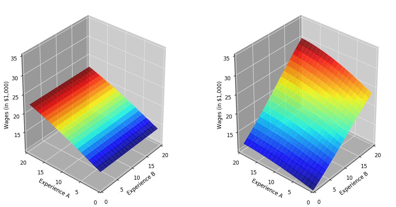
Keane and Wolpin (1994) generate three different Monte Carlo samples. We study their first parameterization in more detail now. We label the two occupations as Occupation A and Occupation B. We first plot the returns to experience. Occupation B is more skill intensive in the sense that own experience has higher return than is the case for Occupation A. There is some general skill learned in Occupation A which is transferable to Occupation B. However, work experience in is occupation-specific in Occupation B.

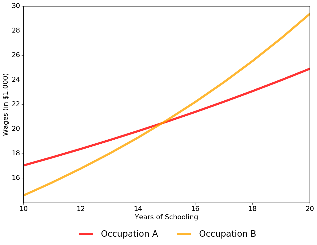
The next figure shows that the returns to schooling are larger in Occupation B. While its initial wage is lower, it does decrease faster with schooling compared to Occupation A.

Simulating a sample of 1,000 agents from the model allows us to study how these features interact in determining agent decisions over their life cycle. Note that all agents start out identically, different choices are simply the cumulative effects of different shocks. Initially, 50% of agents increase their level of schooling but the share of agents enrolled in school declines sharply over time. The share working in Occupation A hovers around 40% at first, but then declines to 21%. Occupation B continuously gains in popularity, initially only 11% work in Occupation B but its share increases to about 77%. Around 1.5% stay at home each period. We visualize this choice pattern in detail below.

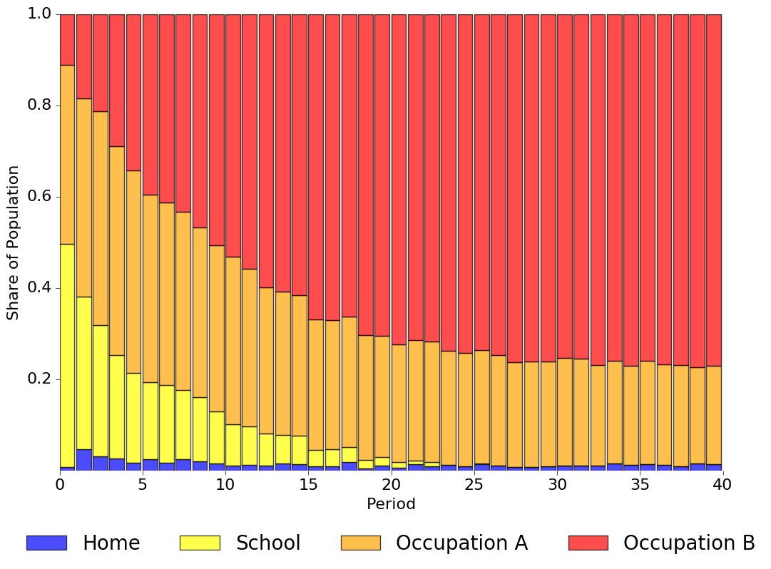
We start out with the large majority of agents working in Occupation A. Eventually, however, most agents ends up working in Occupation B. As the returns to education are higher for Occupation B and previous work experience is transferable, Occupation B gets more and more attractive as agents increase their level of schooling and gain experience in the labor market.